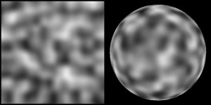
Analytical Noise Derivatives

Procedural noise functions return smoothly varying results as calculated from spatial coordinates (as the spatial coordinate changes so does the value). The derivatives of procedural noise functions can be useful in many different ways.
eg
analytical bump/normal mapping
interesting fractal effects
calculating entirely new noise types

Noise derivatives can be calculated in a number of ways. Ken Perlin gives an example where derivatives are calculated numerically using finite differencing (5.6). An advantage to this is the noise function can be any arbitrarily complex function. Disadvantages are that the noise function needs sampling 3 times and some fixed epsilon value needs to be chosen (eg 0.0001). Hugh Malan shows that for realtime use derivatives can be baked into a texture along with the original value (20.3.1). Although very efficient the disadvantage with this is we’re now locked into a fixed resolution which makes general use problematic.  Morten Mikkelsen shows that GPU hardware derivative units can be used, which is a very nice and efficient solution, but the result suffers from grainy artifacts due to the 2×2 sampling strategy used by derivative hardware.

Another approach is to calculate the derivatives analytically. That is, the procedural noise function calculates both the result and the derivative mathematically in a single call. This has the advantage of only needing to be called once and also being robust when sampled at any scale.

Given the advantages/uses of procedural noise derivatives I’m surprised analytical derivatives have not received much attention at all. I went hunting and found Stefan Gustavson’s work on simplex noise derivatives in C++,  Giliam de Carpentier’s work on 2D Perlin noise derivatives and Milo Yip’s post regarding 3D perlin noise derivatives. With that I went about implementing them myself.  As a result the noise library now contains common noise functions (value, perlin, cellular, hermite and simplex) which also return analytical derivatives.

Here are some screenshots showing some common procedural noise functions with their corresponding derivatives.  Please note that all images have been normalized to a 0.0->1.0 range for ease of viewing.  In reality the noise values range from -1.0->1.0 and noise derivatives can have any range but generally somewhere around -3.0->3.0

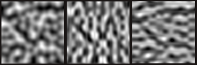
Classic Perlin Noise

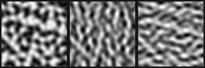
Classic Perlin Noise “Value”, “DerivX” and “DerivY” (notice grid line artifacts)

Hermite Noise

Hermite Noise “Value”, “DerivX” and “DerivY” (notice grid line artifacts greatly reduced)

Simplex Perlin Noise

Simplex Perlin Noise “Value”, “DerivX” and “DerivY” (notice absence of any grid-aligned artifacts)

Posted in Uncategorized | 5 Comments

Adding a 4th dimension

In a previous post I describe a fast 32-bit hash function which I’ve been using as the basis for all noises documented on this site.  Recently I have made some changes to it resulting in…

  • Improved flexibility
  • A slight improvement in randomness
  • A larger possible domain
  • The possibility of a 4D hash function

For anyone interested in the inner workings, the change is that the input coordinate is first scaled before offsetting the domain.  This has allowed for a larger range of precision for the hashing process.  As with the previous hash function, here is some GLSL code which implements the new 32bit hash function to calculate pseudo random 0.0->1.0 hash values for the 4 corners of a 2D integer grid cell.

vec4 FAST32_2_hash_2D( vec2 gridcell )
{
// gridcell is assumed to be an integer coordinate
const vec2 OFFSET = vec2( 403.839172, 377.242706 );
const float DOMAIN = 69.0;
const float SOMELARGEFLOAT = 32745.708984;
const vec2 SCALE = vec2( 2.009842, 1.372549 );
vec4 P = vec4( gridcell.xy, gridcell.xy + 1.0 );
P = P - floor(P * ( 1.0 / DOMAIN )) * DOMAIN;
P = ( P * SCALE.xyxy ) + OFFSET.xyxy;
P *= P;
return fract( P.xzxz * P.yyww * ( 1.0 / SOMELARGEFLOAT ) );
}

The new hash function is slightly slower than the old one so I have left all current noises unchanged.  But given that the new function allows for 4D hashing I have written some new 4D Value and 4D Classic Perlin noises.  Complete source for the improved hash function and these new noises can be found on the GitHub repository.

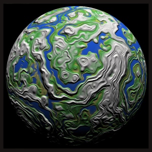
It is always great to show an image at the end of a post, but it is hard to show the benefits of a 4D noise given that the images are not animated.  One great use of 4D noise is through domain distortion (instead of applying a 3D noise over a 3D surface, use a 4D noise and feed an additional noise into the 4D dimension).  The following image shows such an effect applied to the surface of a planet  : )

Planet rendering showing a distorted fractal

Planet rendering showing a distorted fractal

Posted in Uncategorized | Leave a comment

Modifications to Classic Perlin Noise

I have been working with analytical noise derivatives lately and it turns out the analytical derivative of classic perlin noise can get rather involved.

Ken Perlin solved this problem in simplex noise by using radial kernel summation rather than interpolation to combine the gradient results.  It occurred to me this idea can be applied back to classic perlin noise and as a result here’s two modifications to classic perlin noise.

Classic Perlin Surflet Noise

The first modification is simply the replacement of interpolation with radial kernel summation as done in simplex noise.  The result is a noise which looks almost identical but has an easily computable analytical derivative.

Classic Perlin Surflet Offset Noise

After applying the first modification I realized we can now jitter ( randomly offset ) the gradient points to help break the fixed grid structure of classic perlin noise.

An animated gif comparing these changes with the original can be seen here.  An example implementation can be found here.

Posted in Uncategorized | 5 Comments

Hermite Noise

Quintic Hermite Interpolation allows us to interpolate a value with respect to 3 variables.  Its position, velocity and acceleration.  In mathematical terms this translates to the function and its 1st+2nd derivative. More information on Quintic Hermite Interpolation can be found here.

Recall from a previous post that we require an interpolation function to have a 2nd derivative of 0.0 at the start+end points in order to be continuous for bump mapping.  This is where Quintic Hermite Interpolation is useful.  It allows us to explicitly use 0.0 for the start+end acceleration which will generate a C2 continuous curve.  It also allows us to supply whatever we want for velocity giving us control of the gradient at grid lattice points.  If the gradient vectors are normalized we get a look very similar to that of Classic Perlin noise.  Here are some initial observations…

I have uploaded initial 2D+3D implementations of Hermite and ValueHermite Noise to the GitHub repository.  ( like ValuePerlin, ValueHermite is a uniform blend between Value and Hermite noise )

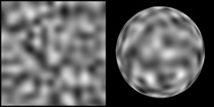
2D+3D sampling of Hermite Noise

2D+3D sampling of Hermite Noise

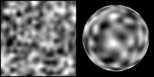
2D+3D sampling of ValueHermiteNoise

2D+3D sampling of ValueHermiteNoise

Posted in Uncategorized | Leave a comment

Simplex Noise

In 2001 Ken Perlin introduced a new type of gradient noise called Simplex Noise.  The document can be found here.  It is essentially his original gradient noise mapped onto a simplex grid.  The term “Simplex” means the simplest possible primitive which can occupy space.  In 2D it is a triangle and in 3D it is a tetrahedron ( 4-sided pyramid ).  A simplex grid is a grid structure made of these primitives.

There are four distinct improvements his new noise had over his classic.

  • A simplex primitive has far fewer verticies than its square/cube equivalent in 2D, 3D and higher dimensions which reduces algorithm complexity.
  • It allows for an easily computable analytic derivative
  • The simplex structure reduces axis-aligned artifacts
  • It lends itself to an efficient hardware implementation

Stefan Gustavson has made some great contributions to Simplex Noise over the years.  Most notably these are…

  • Writing a much clearer description of Simplex Noise in his “Simplex Noise Demystified” document.
  • Along with Ian McEwan providing GLSL implementations of Simplex Noise at WebGLNoise.
  • Providing an implementation of Simplex Noise with analytical derivatives here.

I have been experimenting with implementing this and other noise types over simplex grids.  As a result I have uploaded 3 new noise types to the GitHub repository.

The first is Simplex Perlin Noise in 2D and 3D.  I have made two improvements over what has been supplied by Perlin and Gustavson.  The first is a fix to a bug in the 3D surflet math which would cause discontinuities along the simplex faces, as can be seen here.  The second is providing accurate scaling values to correctly scale the noise to a strict -1.0->1.0 range.

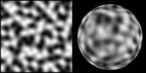
2D+3D sampling of Simplex Perlin Noise  ( simplex gradient noise )

2D+3D sampling of Simplex Perlin Noise ( simplex gradient noise )

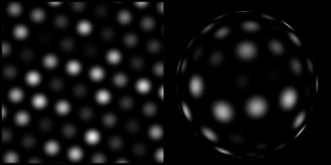
The second is Simplex PolkaDot Noise in 2D and 3D.  The simplex grid packs the dots more tightly than the square/cube version which gives the noise a slightly different look.

2D+3D sampling of Simplex PolkaDot Noise

2D+3D sampling of Simplex PolkaDot Noise

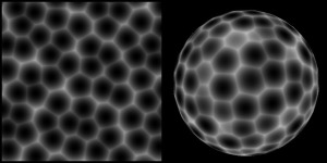
The final is Simplex Cellular Noise in 2D and 3D.  I’ve used some optimization ideas as described in a previous post on Cellular Noise so it runs very efficiently.  And given the reduced complexity in higher dimensions it could run a lot faster than its cube grid alternative.  The problem is a simplex grid packs the points much more tightly in space than a cube grid which reduces area for the verticies to move.  This reduces variance leading to a repetitive looking noise.  Nonetheless it is still visually pleasing and well defined so I have included it into the code repository.

One final note is that I experimented with taking additional points into account ( other than the immediate corner verticies of the simplex ) to allow for more variance.  The results were positive ( as can be seen here ) but costly and would only be of benefit in higher dimensions ( eg 3 or 4 ).

2D+3D sampling of Simplex Cellular Noise

2D+3D sampling of Simplex Cellular Noise

Posted in Uncategorized | 19 Comments

PolkaDot, Star and Cubist Noises

I’ve uploaded three new noise types to the GitHub repository.  The first is a PolkaDot style noise in both 2D and 3D which generates smooth falloff dots at random sizes, intensities and locations over a uniform grid.  ( There’s even a one-line modification which can give square dots instead : ) )

2D+3D sampling of PolkaDot Noise

2D+3D sampling of PolkaDot Noise

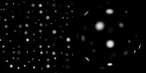
The second is a 2D Stars noise with behavior similar to the PolkaDot noise but which also allows for the possibility that a dot/star be not drawn.  This can generate a sparse distribution of dots which look very suitable for a starry sky.

Sample of 2D Stars Noise

Sample of 2D Stars Noise

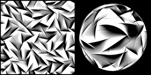
The third is a noise made more for fun.  It is called “cubist” noise due to it resembling a cubist painting style.  The problem is that it contains sharp discontinuities and also a possible range of +-infinity which must be arbitrarily clamped ( eg +- 1.0->5.0 ),  so it is unfit for displacement or distortion but should produce some interesting results when used for texturing.

2D+3D samlping of Cubist Noise

2D+3D samlping of Cubist Noise

Posted in Uncategorized | Leave a comment

Optimized Artifact-Free GPU Cellular Noise

Cellular Noise is a noise basis which mimics a voronoi diagram.  It was first proposed by Steven Worley in his 1996 paper “A Cellular Texture Basis Function” and has been used extensively by the graphics community ever since.

Stefan Gustavson has been doing some great work with optimized GPU Cellular Noise lately at http://webstaff.itn.liu.se/~stegu/GLSL-cellular/.  The usual implementation of 2D Cellular Noise searches over 9 jittered points on a 3×3 grid to find the closest point.  Stefan has optimized it to work with 4 jittered points on a 2×2 grid.  This reduces the work significantly but can create artifacts which show as discontinuities.

I will be using noise in my procedural modeler to create displaced surfaces as well as for solid texturing which mean discontinuities are unacceptable.  So I have decided to continue on from Stefan’s work and create an optimized GPU Cellular Noise which is free from discontinuities.

The artifacts in Stefan’s implementation come from the possibility that closest jittered points may exist outside the 2×2 search region ( which is why Worley uses 3×3 ).  We can eliminate this by reducing the jitter size ( eg from +-0.5 to +-0.25 ) so there can be no way a closest point can exist outside the 2×2 search region.  I did some calculations and found in 2D this distance is +-0.25 and in 3D it is +-0.16666666.  The problem with reducing the jitter distance to such a small amount is the noise has very little variation and the grid structure becomes apparent.

To fix this I use a cubic function to push the randomly placed points outwards to the extremes of the jitter window.  The result is an acceptable-looking artifact-free GPU Cellular Noise which runs at an acceptable speed.  I have uploaded 2D+3D implementations to the GitHub repository.  I have left the original functionality proposed by Stefan in as an option in case the artifacts are acceptable for your own use.

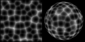
2D+3D sampling of Cellular Noise

2D+3D sampling of Cellular Noise

My next step with this is to explore one of Stefan’s other ideas.  In 2D this is to sample things in a 2.5D manner where the points are jittered over the 2D grid as normal, but also jittered in a 3rd dimension.  A 2D slice is then taken through the center of the 3rd dimension to sample the noise.  This would add more variance to the 2D noise.  The same can be done in 3D.  Jittering would still need to be restricted to ensure a continuous signal but variance may be good enough that cubic weighting is not needed.

Posted in Uncategorized | 7 Comments

GitHub code repository

I always like it when people provide clean implementations of their work which can be dropped easily into a project without much programmer effort.  Stefan Gustavson and Ian McEwan have done this at webgl-noise so I’ve decided to take their lead and do the same.  I’ve created a GitHub repository which can be found here https://github.com/BrianSharpe and also by clicking the “code” button in the blog menu bar above.

The first commit has been of the work so far…

  • BBS, SGPP and FastHash32 hashing implementations
  • C1, C2 and C3 interpolation and falloff functions

Also included are some optimal texture-free 2D + 3D Value, Perlin and ValuePerlin noise implementations.

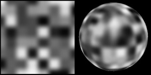
2D+3D sampling of Value Noise

2D+3D sampling of Value Noise

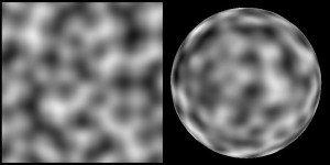
2D+3D sampling of Perlin Noise ( gradient noise )

2D+3D sampling of Perlin Noise ( gradient noise )

2D+3D sampling of ValuePerlin Noise ( value-gradient noise )

2D+3D sampling of ValuePerlin Noise ( value-gradient noise )

Posted in Uncategorized | Leave a comment

A fast and simple 32bit floating point hash function

In a previous post I reviewed two existing floating point hash functions which are suitable for use in fragment shaders.  These were the BlumBlumShub and Permutation Polynomial hash functions used in MNoise and WebGLNoise.  If curious, here is a link to the post https://briansharpe.wordpress.com/2011/10/01/gpu-texture-free-noise/

I’ve become disheartened with both.  They both contain artifacts and are slow to calculate.  The BBS hash is still useful because it can run on 16bit and 24bit floating point hardware.  But now that we have 32bit floating point hardware I’ve decided make a floating point hashing function of my own.

The hash function which is working best for me takes the form hash = mod( coord.x * coord.x * coord.y * coord.y, SOMELARGEFLOAT ) / SOMELARGEFLOAT.  The 3D version simply offsets the SOMELARGEFLOAT value by a fraction of the Z coordinate.  It takes some time to find constants which give good visual results and also to find a specific area of the noise which is most free from artifacts.  It would be good to one day use some kind of computational process to find constants which give the best possible noise, but for now my hand-picked values should work ok.

One thing to note is the x*x*y*y operation pushes the floating point number well over 2^23 causing a loss of precision, which is where a lot of the “randomness” comes from.  Because of this I’m not sure if it will give identical results across cards.  More investigation is required.  But for now its giving good results on my CPU and ATI card so I’m going to stick with it.  : )

As with the previous hash functions, here is some GLSL code which implements the new 32bit hash function to calculate pseudo random 0.0->1.0 hash values for the 4 corners of a 2D integer grid cell.

//
//    FAST_32_hash
//    A very fast 2D hashing function.  Requires 32bit support.
//
//    The hash formula takes the form....
//    hash = mod( coord.x * coord.x * coord.y * coord.y, SOMELARGEFLOAT ) / SOMELARGEFLOAT
//    We truncate and offset the domain to the most interesting part of the noise.
//
vec4 FAST_32_hash( vec2 gridcell )
{
//    gridcell is assumed to be an integer coordinate
const vec2 OFFSET = vec2( 26.0, 161.0 );
const float DOMAIN = 71.0;
const float SOMELARGEFLOAT = 951.135664;
vec4 P = vec4( gridcell.xy, gridcell.xy + 1.0.xx );
P = P - floor(P * ( 1.0 / DOMAIN )) * DOMAIN;    //    truncate the domain
P += OFFSET.xyxy;                                //    offset to interesting part of the noise
P *= P;                                          //    calculate and return the hash
return fract( P.xzxz * P.yyww * ( 1.0 / SOMELARGEFLOAT.x ).xxxx );
}

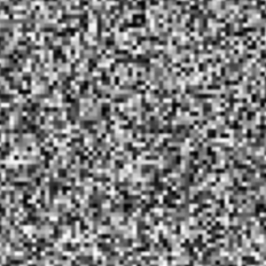
Here is an image showing a 61×61 sampling of the Fast 32bit hashing function  ( 61×61 for comparison with BBS and SGPP, the actual domain is 72×72 ).

A 61x61 sampling of the Fast 32bit floating point hash function

A 61×61 sampling of the Fast 32bit floating point hash function

Posted in Uncategorized | 4 Comments

Useful Interpolation Functions for Noise Development

Interpolation functions allow us to calculate a transition between discreet points.  They are used in noise development.   Here are some common types.

Smooth interpolation of a linear input from 0.0 to 1.0

This is a very common interpolation function.  It calculates a smooth transition from 0.0 to 1.0 as the input increases linearly from 0.0 to 1.0.  By smooth I mean the gradient is 0.0 at 0.0, 0.0 at 1.0 and positive in between.  An example is the GLSL function SmoothStep().

Ken Perlin uses a cubic hermite curve in his original classic noise.  It is of the form f(x) = 3x^2-2x^3.  A problem is that the 2nd derivative is non-zero at 0.0 and 1.0.  This can result in a sharp transition when the noise is used to calculate a normal for shading.  Ken solved the problem with a quintic hermite curve of the form f(x) = 6x^5-15x^4+10x^3.  This new function has both 1st and 2nd derivatives of 0.0 at 0.0 and 1.0.  More details can be found in his paper.  http://mrl.nyu.edu/~perlin/paper445.pdf

The cubic curve is said to be 1st derivative continuous ( C1 for short ).  The quintic curve is said to be 1st and 2nd derivative continuous ( C2 for short ).

Here are 4 implementations of this interpolation function.  The first two are the previously mentioned cubic and quintic curves.  The third is a more efficient C2 interpolation function which contains 1 less multiply than Perlin’s quintic curve.  The forth is a C3 interpolation function.  Their graph can be seen here.

//
//    Interpolation functions
//    ( smoothly increase from 0.0 to 1.0 as x increases linearly from 0.0 to 1.0 )
//

//    Cubic Hermine Curve.  Same as SmoothStep().  As used by Perlin in Original Noise.
//    3x^2-2x^3
float Interpolation_C1( float x ) { return x * x * (3.0 - 2.0 * x); }

//    Quintic Hermite Curve.  As used by Perlin in Improved Noise.  http://mrl.nyu.edu/~perlin/paper445.pdf
//    6x^5-15x^4+10x^3
float Interpolation_C2( float x ) { return x * x * x * (x * (x * 6.0 - 15.0) + 10.0); }

//    Faster than Perlin Quintic.  Not quite as good shape.
//    7x^3-7x^4+x^7
float Interpolation_C2_Fast( float x ) { float x3 = x*x*x; return ( 7.0 + ( x3 - 7.0 ) * x ) * x3; }

//    C3 Interpolation function.  If anyone ever needs it... : )
//    25x^4-48x^5+25x^6-x^10
float Interpolation_C3( float x ) { float xsq = x*x; float xsqsq = xsq*xsq; return xsqsq * ( 25.0 - 48.0 * x + xsq * ( 25.0 - xsqsq ) ); }

Smooth falloff of a squared input from 0.0 to 1.0

A smooth falloff function is a function which decreases from 1.0 to 0.0 as its input increases from 0.0 to 1.0.  To say that it operates on x-squared means that it accepts a squared input rather than a linear one.  They can be used to efficiently fade out from a point due to the avoidance of a sqrt() call.

Listed here are two which are commonly used.  A graph of the functions can be seen here.  Included in the comments are some smooth interpolating functions also defined in x-squared.  Their graph can be seen here.

//
//    Falloff defined in XSquared
//    ( smoothly decrease from 1.0 to 0.0 as xsq increases from 0.0 to 1.0 )
//

// ( 1.0 - x*x )^2 ( Used by Humus for lighting falloff in Just Cause 2. GPUPro 1 )
float Falloff_Xsq_C1( float xsq ) { xsq = 1.0 - xsq; return xsq*xsq; }
// ( 1.0 - x*x )^3. NOTE: 2nd derivative is 0.0 at x=1.0, but non-zero at x=0.0
float Falloff_Xsq_C2( float xsq ) { xsq = 1.0 - xsq; return xsq*xsq*xsq; }

//
//  For interest here are some smooth interpolation functions defined in x-squared
//
//  C1:      f(x) = 1.0 - ( 1.0 - x*x )^2
//  C2:      f(x) = 9x^4-16x^6+9x^8-x^12
//  C2 Fast: f(x) = 5x^4-5x^6+x^10  or  f(x) = 3x^4-3x^8+x^12
//  C3:      f(x) = 10x^4-20x^6+15x^8-4x^10
//
Posted in Uncategorized | 1 Comment